GEO DataSets: Experiment Selection and Initial Processing

A walkthrough of processing bulk RNA-seq data from the GEO database purely in R.

This article demonstrates a pure R workflow of finding experiments of interest, downloading datasets of experiments of interest from the Gene Expression Omnibus (GEO) database, and processing the bulk RNA-seq counts data.

The readers are assumed to have certain degree of understanding of what the GEO database is.

Finding Experiments of Interest

GEO metadata repository: GEOmetadb

GEOmetadb is a thin wrapper around a SQLite database into which all the most up-to-date NCBI GEO metadata that are associated with GEO samples (GSM), GEO platforms (GPL), GEO data series (GSE), and curated GEO datasets (GDS) are parsed.(Zhu et al. 2008) It enables querying the GEO database using R scripts without accessing the webpage. Although NCBI’s public API to the NCBI Entrez system The E-utilities also also offers an option for scripting queries for finding datasets of interest in the GEO database, the E-utilities are difficult to use (e.g. might need HTTP POST calls for long queries) and require extra effort to learn.

To install GEOmetadb via Bioconductor:

if (!requireNamespace("GEOmetadb", quietly = TRUE))
    BiocManager::install("GEOmetadb", ask = FALSE)

We will also create a directory ./data dedicated to storing data files under the working directory:

if(!dir.exists("./data")) {
    dir.create("./data", showWarnings = FALSE)
}

Then we download the SQLite database that has the GEO metadata into ./data via GEOmetadb:

# Download GEOmeta database if not found
metadb <- file.path(".", "data", "GEOmetadb.sqlite")
if(!file.exists(metadb)) {
    ## avoid re-downloading the 11G database everytime running the script
    metadb <- GEOmetadb::getSQLiteFile(destdir = "./data")
}

Querying GEO database

For this demonstration, we are interested in experiments that:

• were done in the recent 6 years
• are studies on COVID-19 (SARS-CoV-2)
• used native human cells or tissues
• have RNA-seq data

To build an query to find experiments that meet the above conditions:

query <- paste(
    "SELECT DISTINCT",
    "gse.title,",
    "gse.gse,",
    "gpl.title AS platform,",
    "gse.submission_date,",
    "gse.supplementary_file",
    "FROM",
    "gse",
    "JOIN gse_gpl ON gse_gpl.gse = gse.gse",
    "JOIN gpl ON gse_gpl.gpl = gpl.gpl",
    "WHERE",
    "gse.submission_date > '2015-01-01' AND",           # not older than 6 years
    "gse.title LIKE '%SARS-CoV-2%' AND ",                  # experiment on COVID
    "gpl.organism LIKE '%Homo sapiens%' AND", # dataset of human cells or tissue
    "gpl.technology LIKE '%high-throughput seq%'")                # RNA-seq data

The ER diagram for the GEOmetadb SQLite database is represented as the following. This might come in useful when constructing an SQL statement querying the database.

The entity-relationship diagram for the GEOmetadb database (Zhu et al. 2008)

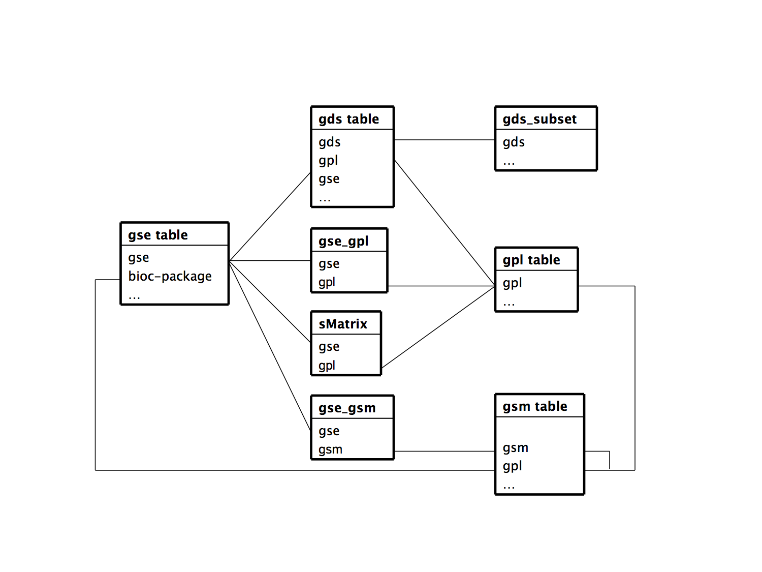
For the GEO accession prefixes present in the figure:

• GSE: Series
  • An original submitter-supplied record that summarizes an experiment
  • links together a group of related Samples and provides a focal point and description of the whole study
  • may also contain tables describing extracted data, summary conclusions, or analyses
• GSM: Sample
  • describes the conditions under which an individual Sample was handled, the manipulations it underwent, and the abundance measurement of each element derived from it
• GPL: Platform
  • composed of a summary description of the array or sequencer and, for array-based Platforms, a data table defining the array template
  • may reference many Samples that have been submitted by multiple submitters
• GDS: DataSet
  • Profiles are derived from DataSets
    • A Profile consists of the expression measurements for an individual gene across all Samples in a DataSet

To establish a connection with the SQLite database:

# Establish connection to GEOmetadb.sqlite
con <- DBI::dbConnect(drv    = RSQLite::SQLite(),   ## an object of SQLiteDriver
                      dbname = metadb)

Note that packages DBI and RSQLite have already been implicitly installed as dependencies for GEOmetadb. Therefore we can directly make the function calls here.

To submit the query to the database:

result <- DBI::dbGetQuery(conn = con, statement = query) ## save query result

Closing connection to the database:

DBI::dbDisconnect(con) ## close connection
rm(con) ## not a necessary step, just wanna keep my workspace clean

Filtering Query Result

The SQL query result is returned as a list object by the wrapper function in R. The result should have the following columns:

names(result)

[1] "title"              "gse"                "platform"          
[4] "submission_date"    "supplementary_file"

We would like to select from only those experiments whose datasets contain RNA-seq count matrices:

hasCounts <- result$supplementary_file[
    grep(
        result$supplementary_file,
        pattern     = "count", ## keyword to look for in experiment data files
        ignore.case = TRUE
        )
    ]

This extracts a vector of FTP links to the files that include RNA-seq counts. Then from the FTP links, we extract the GSE series numbers from their file names using regex:

hasCounts_gse <- unlist(
    regmatches(hasCounts,
               regexec("GSE[0-9]{4,}[^/]", hasCounts)
    )
)
SELECT_ROWS       <- result$gse %in% hasCounts_gse
candidate_dataset <- result[SELECT_ROWS, ]

The GSE series numbers and titles of the qualified candidate experiments (candidate_dataset) that contain RNA-seq data are as follows:

	title	gse
1	Transcriptional response of human lung epithelial cells to SARS-CoV-2 infection	GSE147507
2	SARS-CoV-2 receptor ACE2 is an interferon-stimulated gene in human airway epithelial cells and is detected in specific cell subsets across tissues	GSE148829
3	SARS-CoV-2 receptor ACE2 is an interferon-stimulated gene in human airway epithelial cells and is detected in specific cell subsets across tissues	GSE148829
5	Spectrum of Viral Load and Host Response Seen in Autopsies of SARS-CoV-2 Infected Lungs	GSE150316
9	RNA-Seq of Human iPSC-cardiomyocytes infected with SARS-CoV-2	GSE150392
10	In vivo antiviral host response to SARS-CoV-2 by viral load, sex, and age	GSE152075
12	Severely ill COVID-19 patients display a defective exhaustion program in SARS-CoV-2 reactive CD8+ T cells	GSE153931
13	Primary Human Airway Epithelial Cultures infected with SARS-CoV-2	GSE153970
14	In vivo antiviral host response to SARS-CoV-2 by viral load, sex, and age [dataset II]	GSE154768
15	In vivo antiviral host response to SARS-CoV-2 by viral load, sex, and age [dataset III]	GSE154769
22	Upper airway gene expression differentiates COVID-19 from other acute respiratory illnesses and reveals suppression of innate immune responses by SARS-CoV-2	GSE156063
24	Acute SARS-CoV-2 Infection in a Universal In Vivo Model for Potential Human Pandemic Coronaviruses is Cytopathic and Elicits a Robust and Sustained Host Innate Immune Response	GSE155286
25	Human Pluripotent Stem Cell-Derived Neural Cells and Brain Organoids Reveal SARS-CoV-2 Neurotropism Predominates in Choroid Plexus Epithelium	GSE157852
28	Expression of SARS-CoV-2 receptor ACE2 and coincident host response signature varies by asthma inflammatory phenotype	GSE158752
30	SARS-CoV-2 infected cells present HLA-I peptides from canonical and out-of-frame ORFs	GSE159191
31	SARS-CoV-2 infected cells present HLA-I peptides from canonical and out-of-frame ORFs	GSE159191
34	Cardiomyocytes Infected by SARS-CoV-2 Recruit Cardiotoxic Macrophages [bulk RNA-seq dataset)	GSE151879
35	Cardiomyocytes Infected by SARS-CoV-2 Recruit Cardiotoxic Macrophages [bulk RNA-seq dataset)	GSE151879
42	Identification of required host factors for SARS-CoV-2 infection in human cells [RNA-seq]	GSE159522
44	SARS-CoV-2 infection of primary human lung epithelium for COVID-19 modeling and drug discovery	GSE155518
48	Temporal and Spatial Heterogeneity of Host Response to SARS-CoV-2 Pulmonary Infection [gene expression]	GSE159787
53	Single Nucleus RNA-Seq Multiomic Profiling Reveals Age-Dynamic Regulation of Host Genes Associated with SARS-CoV-2 Infection [scRNA-Seq]	GSE161382
56	Genome-scale identification of SARS-CoV-2 and pan-coronavirus host factor networks	GSE162038
57	Functional interrogation of a SARS-CoV-2 host protein interactome identifies unique and shared coronavirus host factors	GSE162039
58	Metabolic reprogramming and epigenetic changes of vital organs in SARS-CoV-2 induced systemic toxicity	GSE162113
59	Infection of human Nasal Epithelial Cells with SARS-CoV-2 and a 382-nt deletion isolate lacking ORF8 reveals similar viral kinetics and host transcriptional profiles	GSE162131
63	Transcriptomic Similarities and Differences in Host Response between SARS-CoV-2 and Other Viral Infection	GSE152641
64	Bulk RNA sequencing of SARS-CoV-2 infected alveolar type I- and type II like cells	GSE153218
73	Identification of Drugs Blocking SARS-CoV-2 Infection using Human Pluripotent Stem Cell-derived Colonic Organoids	GSE148696
74	Response to SARS-CoV-2 infection in cornea, limbus and sclera from human donors	GSE164073
76	Dysregulated transcriptional responses to SARS-CoV-2 in the periphery support novel diagnostic approaches	GSE161731
78	A Multiplexed, Next-Generation Sequencing Platform for High-Throughput Detection of SARS-CoV-2 [PoC cohort]	GSE160031
79	A Multiplexed, Next-Generation Sequencing Platform for High-Throughput Detection of SARS-CoV-2 [test cohort]	GSE160032
80	A Multiplexed, Next-Generation Sequencing Platform for High-Throughput Detection of SARS-CoV-2 [pilot cohort]	GSE160033
81	A Multiplexed, Next-Generation Sequencing Platform for High-Throughput Detection of SARS-CoV-2 [extended cohort]	GSE160034
84	SARS-CoV-2 infection of human pancreatic islets	GSE159717
94	Expression profiling of SARS-CoV-2 infected patients by RNA-seq	GSE154244

We choose GSE152641 from the candidate studies to be our experiment of interest for the following demonstration.

series <- "GSE152641" ## GEO series ID

Always read the publication of the original experiment and understand the experiment before starting the analysis.

Overview of the chosen experiment

The original study of GSE152641(Thair et al. 2021) performed expression analysis on genes of these 86 samples and compiled expression data of prior studies on six viruses: influenza, RSV, HRV, Ebola, Dengue, and SARS in an attempt to isolate COVID-19 biomarkers from other viral infections. The RNA-seq data was generated by profiling peripheral blood from 62 COVID-19 patients and 24 healthy controls via bulk RNA-seq. The RNA-seq count matrix in the data file consists of 20460 unique Entrez gene IDs along the rows and 86 samples (biological replicates) along the columns.

Downloading Dataset

GEOquery provides easy and quick methods for accessing data from GEO (Davis and Meltzer 2007):

if (!requireNamespace("GEOquery", quietly = TRUE))
    BiocManager::install("GEOquery", ask = FALSE)

To download the RNA-seq data file for the corresponding GSE series number from GEO:

## Get names of data files
fname <- GEOquery::getGEOSuppFiles(GEO           = series,
                                   fetch_files   = FALSE,  ## Don't download yet
                                   makeDirectory = FALSE)$fname

## Download the dataset if it's never downloaded into the data directory
if (!file.exists(file.path(getwd(), "data", fname))) {
    GEOquery::getGEOSuppFiles(GEO           = series,
                              baseDir       = "./data",
                              makeDirectory = FALSE)
}

The dataset file has been downloaded in ./data. Note that this experiment has only 1 supplementary file; some experiments could have more than just one. Therefore you might want to check what’s in fname or look up the GEO accession viewer before proceeding.

RNA-seq Counts Normalisation

Normalising RNA-seq counts is a necessary step of initial data processing prior to the differential expression analysis. The reason is that direct comparison of raw count values does not account for the effects of factors that introduce systematic errors such as different gene lengths and GC-content between genes within a biological replicate, different sequencing depth between biological replicates, and true biological differences in RNA composition between biological replicates, which have a significant impact on downstream analysis (e.g. differential expression analysis). The goal of normalisation is to minimise the effects of systematic errors by taking into account these factors.

There exist various normalisation methods. They come with different assumptions and correct for different factors. Evans, C., Hardin, J., and Stoebel, D. M. have published a detailed review on several common normalisation methods (DESeq, Med, Q, RPKM and ERPKM, TMM, UQ) and discussed how to choose the appropriate normalisation method based on their assumptions. (Evans, Hardin, and Stoebel 2016)

Here we use the trimmed mean of M-values (TMM) normalisation method implemented in edgeR (Mark D. Robinson, McCarthy, and Smyth 2009)(McCarthy, Chen, and Smyth 2012a):

if (!requireNamespace("edgeR", quietly = TRUE))
    BiocManager::install("edgeR", ask = FALSE)

TMM Normalisation

The TMM approach assumes the majority of genes are not differentially expressed. It takes into account sequencing depth, gene length, and RNA composition, making the normalised count values comparable within and between samples. Readers can consult the original publication of TMM normalisation for complete details of this method. (Mark D. Robinson and Oshlack 2010)

The following normalisation procedure is based on the edgeR differential expression analysis protocol, step 14. i-v. (Anders et al. 2013)

Loading dataset

covid19_exp <- read.csv(
    file        = file.path(".", "data", fname),
    header      = TRUE,
    check.names = FALSE ## prevent R from messing up column names
)

To view the first 5 genes of the count matrix:

	IMX_sample00001	IMX_sample00002	IMX_sample00003	IMX_sample00004	IMX_sample00005	IMX_sample00006	IMX_sample00007	IMX_sample00008	IMX_sample00009	IMX_sample00010	IMX_sample00011	IMX_sample00012	IMX_sample00013	IMX_sample00014	IMX_sample00015	IMX_sample00016	IMX_sample00017	IMX_sample00018	IMX_sample00019	IMX_sample00020	IMX_sample00021	IMX_sample00022	IMX_sample00023	IMX_sample00024	IMX_sample00025	IMX_sample00026	IMX_sample00027	IMX_sample00028	IMX_sample00029	IMX_sample00030	IMX_sample00031	IMX_sample00032	IMX_sample00033	IMX_sample00034	IMX_sample00035	IMX_sample00036	IMX_sample00037	IMX_sample00038	IMX_sample00039	IMX_sample00040	IMX_sample00041	IMX_sample00042	IMX_sample00043	IMX_sample00044	IMX_sample00045	IMX_sample00046	IMX_sample00047	IMX_sample00048	IMX_sample00049	IMX_sample00050	IMX_sample00051	IMX_sample00052	IMX_sample00053	IMX_sample00054	IMX_sample00055	IMX_sample00056	IMX_sample00057	IMX_sample00058	IMX_sample00059	IMX_sample00060	IMX_sample00061	IMX_sample00062	IMX_sample00063	IMX_sample00064	IMX_sample00065	IMX_sample00066	IMX_sample00067	IMX_sample00068	IMX_sample00069	IMX_sample00070	IMX_sample00071	IMX_sample00072	IMX_sample00073	IMX_sample00074	IMX_sample00075	IMX_sample00076	IMX_sample00077	IMX_sample00078	IMX_sample00079	IMX_sample00080	IMX_sample00081	IMX_sample00082	IMX_sample00083	IMX_sample00084	IMX_sample00085	IMX_sample00086
1	12	1	10	12	4	12	7	14	19	11	3	11	10	7	11	27	7	4	15	9	8	8	8	5	2	5	0	2	3	12	0	10	3	3	1	7	7	7	5	0	3	0	0	2	6	11	0	6	6	1	3	0	9	7	0	13	2	13	1	0	4	7	6	2	11	2	4	4	8	6	1	1	5	5	0	0	2	0	2	3	1	4	10	0	1	4
2	2670	2432	781	2381	2622	3273	3969	2597	1692	2571	898	1405	1132	1255	1560	585	1075	925	2989	6413	999	3950	2192	2810	829	1461	900	1261	191	1113	57	1609	2674	242	776	996	904	837	943	543	1669	651	259	1177	954	1871	553	1368	646	1607	1021	269	1323	1039	471	738	872	2245	989	2009	591	656	107	338	1285	850	861	3560	4959	1602	1696	1328	1419	475	369	736	351	1327	1458	557	591	824	643	1403	393	1009
9	77	129	87	98	81	86	124	74	68	103	82	104	54	66	50	31	81	112	347	192	192	135	94	122	153	194	129	130	80	273	53	140	96	90	91	79	108	131	100	91	54	96	68	104	62	101	100	119	137	94	88	99	97	144	101	95	112	107	71	72	76	125	81	148	125	98	113	111	96	101	76	122	140	84	121	106	59	134	90	141	75	59	82	91	48	25
10	0	0	0	0	0	0	9	0	2	2	4	0	0	3	0	0	2	0	1	5	0	0	0	0	0	0	0	1	2	8	0	2	2	1	0	0	0	14	1	0	1	0	0	3	0	0	2	0	0	10	7	0	1	0	3	9	2	3	2	0	6	3	0	0	0	6	0	3	1	5	4	0	4	0	0	3	1	11	1	0	0	0	0	3	0	0
12	0	4	0	0	0	1	0	6	5	0	4	0	0	5	0	0	2	1	0	7	0	2	0	0	5	7	0	0	3	6	1	0	0	2	0	0	0	0	1	0	0	0	4	1	0	3	0	0	0	0	4	2	4	0	12	4	1	3	0	0	0	5	0	5	0	2	0	12	3	5	0	3	1	1	3	1	5	0	1	0	0	3	0	0	0	0

Note that the name for the column of gene IDs is blank. Label the column to avoid confusion:

colnames(covid19_exp)[1] <- "entrezgene_id" ## genes were labeled w/ Entrez IDs

Defining group

This is an experiment with a simple design: a simple comparison between two sample groups: COVID-19 and healthy control.(Thair et al. 2021)

For most experiments in the GEO database, groups to which samples belong are usually indicated in samples’ titles. This means we are able to define groups for samples using regex to check their titles, which are the column names of the count matrix.

It used to be the case for GSE152641. Samples that are in the healthy control group had BRH or HMN prefix in their titles, and those in the COVID-19 group had ESC prefix. However, the author of GSE152641 recently replaced the prefix in all of the samples’ title with IMX_sample; in fact they changed the whole samples’ titles. This means we can no longer identify samples’ groups from their titles. The only way to find out their groups is look up their GSM accession numbers. Indeed, checking them one at a time on the GEO accession viewer and manually grouping them are lame.

We can again turn to GEOquery for retrieving samples’ metadata associated with their GSM accession numbers:

gse <- GEOquery::getGEO(GEO = series, GSEMatrix = FALSE)
gsm <- GEOquery::GSMList(gse)

The metadata of the experiment GSE152641 in the GEO database is in the SOFT format. GEOquery can parse the metadata of GSE152641 into GSE class, and each sample’s GSM data is in the list under the GSE object.

To view the first 5 samples’ GSM accession numbers:

head(names(gsm), n = 5)

[1] "GSM4622627" "GSM4622628" "GSM4622629" "GSM4622630" "GSM4622631"

And the metadata that we need from the first sample:

GEOquery::Meta(gsm[[1]])[c(2, 31)]

$characteristics_ch1
[1] "disease: Healthy control" "tissue: Whole blood"     
[3] "age: 46"                  "Sex: Male"               

$title
[1] "IMX_sample00001"

Knowing these two pieces of information for each sample of the experiment, we are now able to define groups for the samples in R. The most R-ish way I’ve come up with so far without using a for-loop:

samples <- lapply(gsm,
                  function(x) {
                      group  <- unlist(
                          regmatches(GEOquery::Meta(x)$characteristics_ch1[1],
                                     regexec(
                                         pattern = "(\\s).*",  ## match by space
                                         GEOquery::Meta(x)$characteristics_ch1[1])
                                     )
                          )[1] ## using regex to extract sample group
                      ## remove space at the beginning of a string
                      group  <- gsub(pattern = "^\\s", "", group)
                      sample <- GEOquery::Meta(x)$title
                      return(
                          data.frame(
                              sample      = sample,
                              group       = group,
                              check.names = FALSE
                              )
                          )
                    }
                  )
samples <- do.call(rbind, samples) ## combine the elements of a list

	sample	group
GSM4622627	IMX_sample00001	Healthy control
GSM4622628	IMX_sample00002	Healthy control
GSM4622629	IMX_sample00003	Healthy control
GSM4622630	IMX_sample00004	Healthy control
GSM4622631	IMX_sample00005	Healthy control
GSM4622632	IMX_sample00006	Healthy control
GSM4622633	IMX_sample00007	Healthy control
GSM4622634	IMX_sample00008	Healthy control
GSM4622635	IMX_sample00009	Healthy control
GSM4622636	IMX_sample00010	Healthy control
GSM4622637	IMX_sample00011	Healthy control
GSM4622638	IMX_sample00012	Healthy control
GSM4622639	IMX_sample00013	Healthy control
GSM4622640	IMX_sample00014	Healthy control
GSM4622641	IMX_sample00015	Healthy control
GSM4622642	IMX_sample00016	Healthy control
GSM4622643	IMX_sample00017	Healthy control
GSM4622644	IMX_sample00018	Healthy control
GSM4622645	IMX_sample00019	COVID19
GSM4622646	IMX_sample00020	COVID19
GSM4622647	IMX_sample00021	COVID19
GSM4622648	IMX_sample00022	COVID19
GSM4622649	IMX_sample00023	COVID19
GSM4622650	IMX_sample00024	COVID19
GSM4622651	IMX_sample00025	COVID19
GSM4622652	IMX_sample00026	COVID19
GSM4622653	IMX_sample00027	COVID19
GSM4622654	IMX_sample00028	COVID19
GSM4622655	IMX_sample00029	COVID19
GSM4622656	IMX_sample00030	COVID19
GSM4622657	IMX_sample00031	COVID19
GSM4622658	IMX_sample00032	COVID19
GSM4622659	IMX_sample00033	COVID19
GSM4622660	IMX_sample00034	COVID19
GSM4622661	IMX_sample00035	COVID19
GSM4622662	IMX_sample00036	COVID19
GSM4622663	IMX_sample00037	COVID19
GSM4622664	IMX_sample00038	COVID19
GSM4622665	IMX_sample00039	COVID19
GSM4622666	IMX_sample00040	COVID19
GSM4622667	IMX_sample00041	COVID19
GSM4622668	IMX_sample00042	COVID19
GSM4622669	IMX_sample00043	COVID19
GSM4622670	IMX_sample00044	COVID19
GSM4622671	IMX_sample00045	COVID19
GSM4622672	IMX_sample00046	COVID19
GSM4622673	IMX_sample00047	COVID19
GSM4622674	IMX_sample00048	COVID19
GSM4622675	IMX_sample00049	COVID19
GSM4622676	IMX_sample00050	COVID19
GSM4622677	IMX_sample00051	COVID19
GSM4622678	IMX_sample00052	COVID19
GSM4622679	IMX_sample00053	COVID19
GSM4622680	IMX_sample00054	COVID19
GSM4622681	IMX_sample00055	COVID19
GSM4622682	IMX_sample00056	COVID19
GSM4622683	IMX_sample00057	COVID19
GSM4622684	IMX_sample00058	COVID19
GSM4622685	IMX_sample00059	COVID19
GSM4622686	IMX_sample00060	COVID19
GSM4622687	IMX_sample00061	COVID19
GSM4622688	IMX_sample00062	COVID19
GSM4622689	IMX_sample00063	COVID19
GSM4622690	IMX_sample00064	COVID19
GSM4622691	IMX_sample00065	COVID19
GSM4622692	IMX_sample00066	COVID19
GSM4622693	IMX_sample00067	COVID19
GSM4622694	IMX_sample00068	COVID19
GSM4622695	IMX_sample00069	COVID19
GSM4622696	IMX_sample00070	COVID19
GSM4622697	IMX_sample00071	COVID19
GSM4622698	IMX_sample00072	COVID19
GSM4622699	IMX_sample00073	COVID19
GSM4622700	IMX_sample00074	COVID19
GSM4622701	IMX_sample00075	COVID19
GSM4622702	IMX_sample00076	COVID19
GSM4622703	IMX_sample00077	COVID19
GSM4622704	IMX_sample00078	COVID19
GSM4622705	IMX_sample00079	COVID19
GSM4622706	IMX_sample00080	COVID19
GSM4622707	IMX_sample00081	Healthy control
GSM4622708	IMX_sample00082	Healthy control
GSM4622709	IMX_sample00083	Healthy control
GSM4622710	IMX_sample00084	Healthy control
GSM4622711	IMX_sample00085	Healthy control
GSM4622712	IMX_sample00086	Healthy control

Save this data frame as an R object. We will need to use it later when performing differential gene expression analysis:

saveRDS(object = samples, file = file.path(".", "data", "samples.rds"))

Normalising counts

Create a numeric matrix of the read counts with the gene IDs as row names:

counts           <- as.matrix(covid19_exp[2:87])
rownames(counts) <- covid19_exp$entrezgene_id

According to the edgeR differential expression analysis protocol(Anders et al. 2013):

“it is recommended to remove features without at least 1 read per million in n of the samples, where n is the size of the smallest group of replicates”

The reason is that a gene must be expressed at some minimal level before it can be translated into a protein. This means genes with very low counts across all libraries provide little evidence for differential expression.

Since we have only two groups: 24 healthy human controls and 62 COVID-19 patients, 24 is the size is the smallest group of biological replicates here:

cpms <- edgeR::cpm(counts)
keep <- rowSums(cpms > 1) >= 24

Or alternatively, by the Bioconductor edgeR user guide:

keep <- edgeR::filterByExpr(cpms, group = samples$group)

It ultimately comes down to users’ preferences for whichever method to use; they produce the same result.

And we only keep genes that meet the threshold of at least 1 read per million in 24 of the samples:

counts <- counts[keep, ]

edgeR stores data in its own data class DGEList and performs analyses on it. Hence we need to first create a DGEList to store the read counts.

Note that although the edgeR documentation says the DGEList constructor takes a numeric matrix for its counts argument, the edgeR user guide says the counts argument can take either a matrix or a data.frame object.

d <- edgeR::DGEList(
  counts = counts,
  group  = samples$group ## add the grouping factor
  )

To estimate the scale factors between samples for TMM normalization:

d <- edgeR::calcNormFactors(d)

Extract the normalised count matrix:

normalised_counts <- edgeR::cpm(d)

Save the normalised count matrix as an R object for later analyses:

saveRDS(object = normalised_counts,
        file   = file.path(".", "data", "normalised_counts.rds"))

Distribution for read counts - Before vs. after normalisation

Even though we are comparing the distributions for pre-normalised read counts and post-normalised read counts, we still normalise the pre-normalised read counts to counts per million (CPM) to account for differences in library sizes between samples for a comparable result. More precisely, we are comparing the distributions for two-fold changes in expression before and after TMM normalisation. Note that genes that were previously removed according to the protocol are also excluded in this comparison.

Show code

par(mfrow = c(1, 2))

boxplot(log2(counts),
        xlab     = "Samples",
        ylab     = "log2 CPM",
        las      = 2,
        cex      = 0.5,
        cex.lab  = 0.75,
        cex.axis = 0.25,
        main     = "Before TMM Normalisation",
        cex.main = 0.75)

#draw the median on each box plot
abline(h   = median(apply(log2(counts), MARGIN = 2, FUN = median)),
       col = "green",
       lwd = 0.75,
       lty = 2)

boxplot(log2(normalised_counts),
        xlab     = "Samples",
        ylab     = "log2 CPM",
        las      = 2,
        cex      = 0.5,
        cex.lab  = 0.75,
        cex.axis = 0.25,
        main     = "After TMM Normalisation",
        cex.main = 0.75)
# draw the median on each box plot
abline(h   = median(apply(log2(normalised_counts), MARGIN = 2,FUN = median)),
       col = "green",
       lwd = 0.75,
       lty = 2)

Show code

par(mfrow = c(1, 2))

log2CPM_density <- apply(log2(counts),
                         MARGIN = 2,
                         FUN    = density)

## Get the normalised fold change cpm
normalised_log2CPM_density <- apply(log2(normalised_counts),
                                    MARGIN = 2,
                                    FUN    = density)

## Calculate the limits across all the samples
xlim <- 0; ylim <- 0
for (i in seq_along(log2CPM_density)) {
    xlim <- range(c(xlim, log2CPM_density[[i]]$x))
    ylim <- range(c(ylim, log2CPM_density[[i]]$y))
}
for (i in seq_along(normalised_log2CPM_density)) {
    xlim <- range(c(xlim, normalised_log2CPM_density[[i]]$x))
    ylim <- range(c(ylim, normalised_log2CPM_density[[i]]$y))
}

## 86 line colours for all 86 samples
cols <- rainbow(length(log2CPM_density))
## choose line type 1 for density graphs of all 86 samples
ltys <- rep(1, length(log2CPM_density))

## Initialize the density plot without density lines
plot(log2CPM_density[[1]],
     xlim     = xlim,
     ylim     = ylim,
     type     = "n",
     ylab     = "Smoothing density of log2-CPM",
     main     = "Before TMM normalisation",
     cex.main = 0.7,
     cex.lab  = 0.75
     )
## Plot smoothing density for each sample
for (i in seq_along(log2CPM_density)) {
    lines(log2CPM_density[[i]],
          col = cols[i])
    }
## Create legend for samples
legend("topright",
       colnames(counts),
       col      = cols,
       lty      = ltys,
       cex      = 0.15,
       border   = "blue",
       text.col = "green4",
       merge    = TRUE,
       bg       = "gray90")





## Initialize the density plot without density lines
plot(normalised_log2CPM_density[[1]],
     xlim     = xlim,
     ylim     = ylim,
     type     = "n",
     ylab     = "Smoothing density of log2-CPM",
     main     = "After TMM normalisation",
     cex.main = 0.65,
     cex.lab  = 0.75,
     )

## Plot smoothing density for each sample
for (i in seq_along(normalised_log2CPM_density)) {
    lines(normalised_log2CPM_density[[i]],
          col = cols[i])
    }
## Create legend for samples
legend("topright",
       colnames(normalised_counts),
       col      = cols,
       lty      = ltys,
       cex      = 0.15,
       border   = "blue",
       text.col = "green4",
       merge    = TRUE,
       bg       = "gray90")

The medians of distributions for normalised RNA-seq counts are much closer to each other. The interquartile ranges for the gene expression levels of each sample also become more consistent after normalisation applied. This means 50% of gene expression levels have similar distributions for each sample.

Post-normalisation Analysis

Biological coefficient of variation (BCV)

To capture the variability in gene expressions between sample groups, we use group as target to build a model matrix:

model_design <- model.matrix(~group, data = samples)

	(Intercept)	groupHealthy control
GSM4622627	1	1
GSM4622628	1	1
GSM4622629	1	1
GSM4622630	1	1
GSM4622631	1	1
GSM4622632	1	1
GSM4622633	1	1
GSM4622634	1	1
GSM4622635	1	1
GSM4622636	1	1
GSM4622637	1	1
GSM4622638	1	1
GSM4622639	1	1
GSM4622640	1	1
GSM4622641	1	1
GSM4622642	1	1
GSM4622643	1	1
GSM4622644	1	1
GSM4622645	1	0
GSM4622646	1	0
GSM4622647	1	0
GSM4622648	1	0
GSM4622649	1	0
GSM4622650	1	0
GSM4622651	1	0
GSM4622652	1	0
GSM4622653	1	0
GSM4622654	1	0
GSM4622655	1	0
GSM4622656	1	0
GSM4622657	1	0
GSM4622658	1	0
GSM4622659	1	0
GSM4622660	1	0
GSM4622661	1	0
GSM4622662	1	0
GSM4622663	1	0
GSM4622664	1	0
GSM4622665	1	0
GSM4622666	1	0
GSM4622667	1	0
GSM4622668	1	0
GSM4622669	1	0
GSM4622670	1	0
GSM4622671	1	0
GSM4622672	1	0
GSM4622673	1	0
GSM4622674	1	0
GSM4622675	1	0
GSM4622676	1	0
GSM4622677	1	0
GSM4622678	1	0
GSM4622679	1	0
GSM4622680	1	0
GSM4622681	1	0
GSM4622682	1	0
GSM4622683	1	0
GSM4622684	1	0
GSM4622685	1	0
GSM4622686	1	0
GSM4622687	1	0
GSM4622688	1	0
GSM4622689	1	0
GSM4622690	1	0
GSM4622691	1	0
GSM4622692	1	0
GSM4622693	1	0
GSM4622694	1	0
GSM4622695	1	0
GSM4622696	1	0
GSM4622697	1	0
GSM4622698	1	0
GSM4622699	1	0
GSM4622700	1	0
GSM4622701	1	0
GSM4622702	1	0
GSM4622703	1	0
GSM4622704	1	0
GSM4622705	1	0
GSM4622706	1	0
GSM4622707	1	1
GSM4622708	1	1
GSM4622709	1	1
GSM4622710	1	1
GSM4622711	1	1
GSM4622712	1	1

Show code

d <- edgeR::estimateDisp(d, design = model_design)
edgeR::plotBCV(d, col.tagwise = "black", col.common = "red",
               main = "Common and Tag-wise Dispersion vs Expression Levels")

edgeR models gene counts with the negative binomial distribution, which assumes the variance of gene counts depends on two dispersion parameters, one of which is the negative binomial dispersion, which describes how much variance deviates from the mean, and the BCV is the square root of this dispersion parameter under the negative binomial model.

The BCV plot presents the estimated relative variability of expression between biological replicates; it illustrates the association between the biological CV and the average true gene abundance.

The common dispersion line suggests all gene expression values vary by close to a BCV value of 0.5 among replicates.(McCarthy, Chen, and Smyth 2012b) The tag-wise dispersion shows BCV values calculated individually for each gene. We observe that genes with higher true abundance (under the assumption that RNA-seq counts follow a negative binomial distribution) have lower BCV’s than genes with lower abundance. This implies that the higher the true expression level of a gene has, the lower its variation in our samples.

Mean-variance relationship

Show code

edgeR::plotMeanVar(
    object                       = d,
    show.raw.vars                = TRUE,
    show.tagwise.vars            = TRUE,
    NBline                       = TRUE,
    show.ave.raw.vars            = TRUE,
    show.binned.common.disp.vars = TRUE,
    main                         = paste(
        "Mean-variance Relationship for 14425 Genes of",
        "COVID-19 Group and Healthy Control Group"),
    cex.main                     = 0.8
)

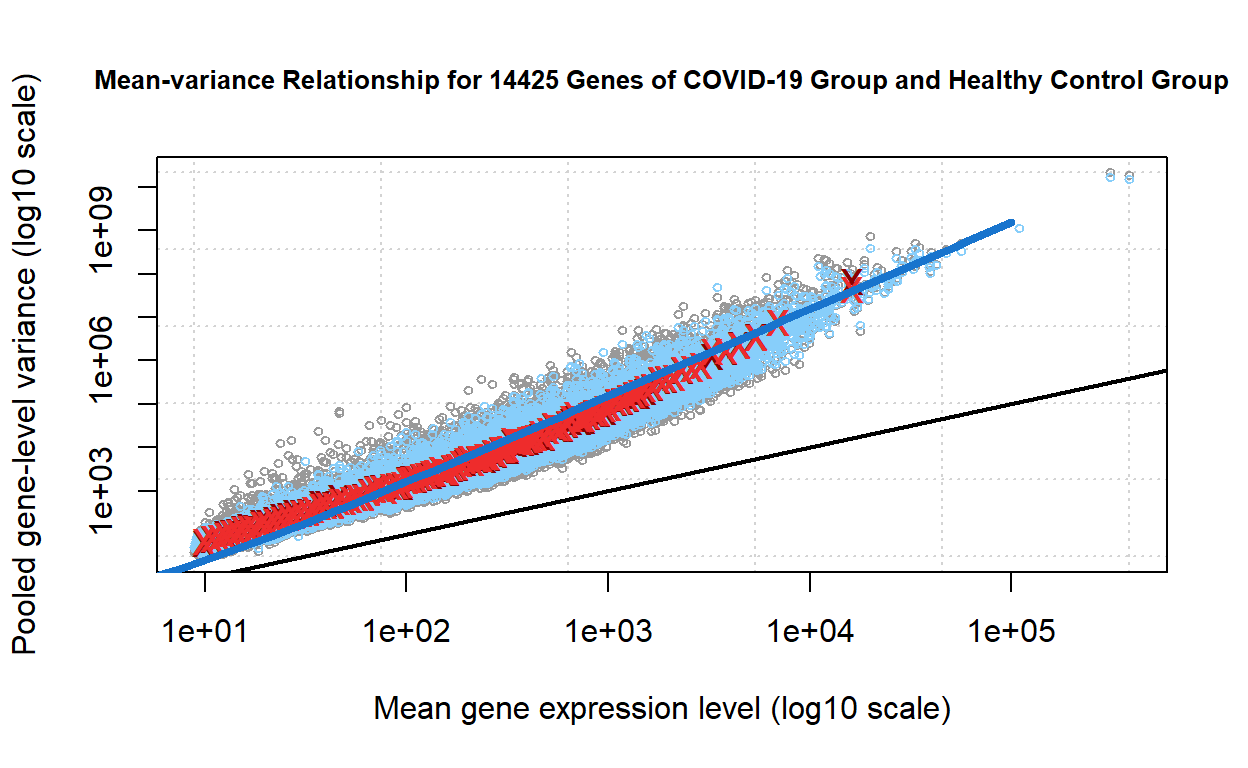
The mean-variance plot presents the modelling of the mean-variance relationship for the normalised expression values, which are split into bins by overall expression level in the model. The grey points represent the pooled gene-wise variances. The blue points on the mean-variance plot represent the estimated gene-wise variances. The red crosses represent the pooled gene-wise variances, while the dark red crosses represent the the average of the pooled variances for each bin of genes plotted against the average expression level of the genes in the bin. The blue line shows the mean-variance relationship for a negative binomial model with common dispersion.(Mark D. Robinson, McCarthy, and Smyth 2009)(McCarthy, Chen, and Smyth 2012a) We observe that all types of variances fit well along the negative binomial line.

Sample relations

Show code

edgeR::plotMDS.DGEList(
    d,
    col      = c("#b7371d", "#51af84")[factor(samples$group)],
    main     = paste("Variation between Samples in Expression Level"),
    cex.main = 1,
    cex      = 0.5,
    cex.axis = 0.75,
    cex.lab  = 0.75
    )
legend("topleft",
       lwd      = 2,
       text.col = c("#51af84","#b7371d"),
       legend   = c("Healthy control", "COVID19"),
       lty      = 0,
       cex      = 0.5)

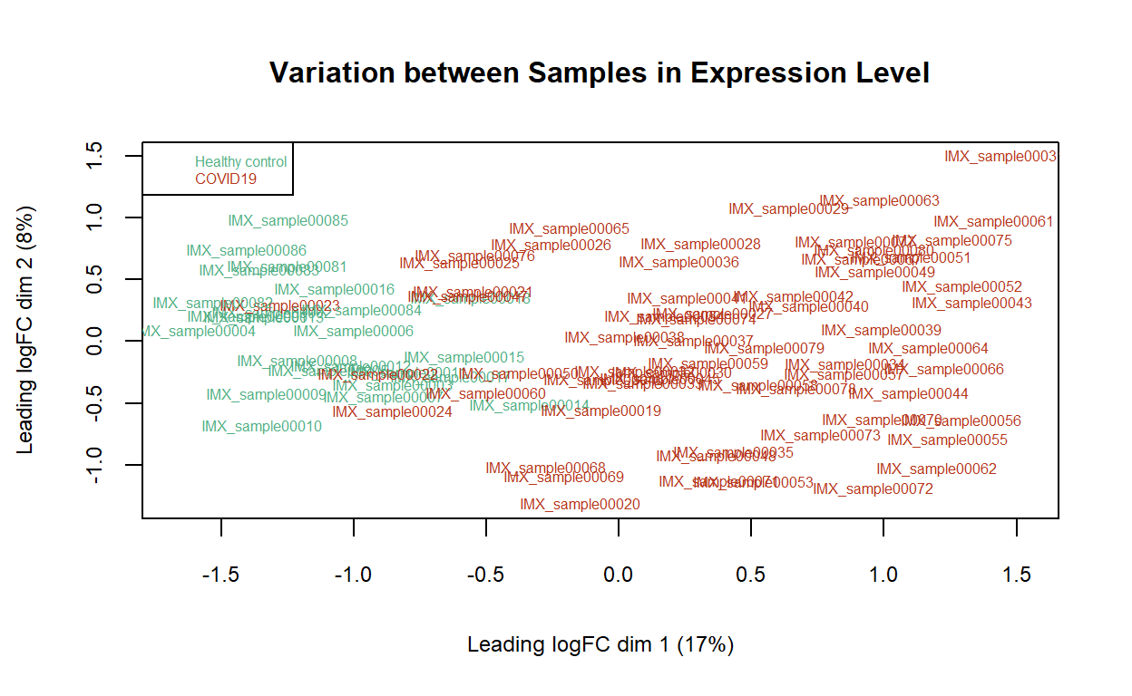
The MDS plot presents variation among samples based on the normalised gene expression. The distances between each pair of samples on the MDS plot suggest how different these samples are in terms of log fold changes of the expression levels of the filtered genes. The healthy control and the COVID-19 patient samples form separate clusters along the plot in the leading logFC dimension 1.

To Do

As the genes in this dataset were labeled with Entrez gene IDs, before performing any further analyses with the processed RNA-seq data, we need to map them to their HGNC names, which are how genes are referred in most annotation datasets and literatures, and more meaningful than simply numerical IDs. This step is supposed to be part of the initial processing; however, mappings produced by different databases vary in quality. I will compare the mapping results produced by 3 different databases and finish converting gene IDs in a later post.